Plotting Text Frequency and Distribution using R for Spinoza's A Theological-Political Treatise [Part I]

This was a little bit of fun, after reading a few more chapters of Text Analysis with R for Students of Literature. Spinoza is a current interest, as I am also reading Radical Enlightenment: Philosophy and the Making of Modernity 1650-1750.

Example Code (Common to Subsections)

 # Text for this can be acquired as below Project Gutenberg, as below
 # http://www.gutenberg.org/cache/epub/989/pg989.txt,
 # or via a Sample Data at the end of this post:
 textToRead = 'pg989.txt'
 
 # Text for this can be acquired via Matthew Jockers site, as below,
 # http://www.matthewjockers.net/macroanalysisbook/expanded-stopwords-list/,
 # or via a Sample Data at the end of this post:
 exclusionFile = 'StopList_Extended.csv'
  
 # Read Text  
 text.scan <- scan(file = textToRead, what = 'char')  
 text.scan <- tolower(text.scan)  
   
 # Create list  
 text.list <- strsplit(text.scan, '\\W+', perl = TRUE)  
 text.vector <- unlist(text.list)  
 
 # Create exclusion list  
 exclusion.file <- scan(exclusionFile, what='char')  
 exclusion.v <- strsplit(exclusion.file, ',', perl = TRUE)  
 exclusion.v <- tolower(exclusion.v)  
   
 # Remove exclusions
 not.exclusions.v <- which(!text.vector %in% exclusion.v)  
 text.vector <- text.vector[not.exclusions.v] 

 # Create sorted list  
 text.frequency = table(text.vector)  
 text.frequency.sorted = sort(text.frequency, decreasing = TRUE)  

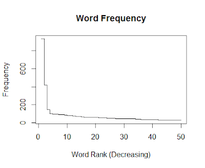
Example Code for Frequency Plot

 # Plots  
 # Types: p = point, l = line, b = both, h = hist, s = stairs  
 plot(text.frequency.sorted[1:50]  
   , type="s"   
   , main = "Word Frequency"  
   , xlab = "Word Rank (Decreasing)"  
   , ylab = "Frequency")

Example Code for Dispersion Plots

 n.time.v = seq(1:length(text.vector))  
   
 textToPlot = 'Spinoza\'s A Theological-Political Treatise [Part I]'  
 wordToPlot = 'god'  
 wordToPlot = 'law'  
 wordToPlot = 'prophets'  
 wordToPlot = 'lord'  
   
 word.v <- which(text.vector == wordToPlot)  
 w.count.v <- rep(NA, length(n.time.v))  
 w.count.v[word.v] <- 1  
   
 plot(w.count.v  
   , main = paste('Dispersion Plot of', wordToPlot, 'in', textToPlot, sep = " ")  
   , xlab = "Document Time"  
   , ylab = wordToPlot  
   , type = "h"  
   , ylim = c(0, 1), yaxt = 'n')  

Sample Data