Posts

Showing posts with the label politics

Support Vector Machines on Big Five Traits and Politics
Image
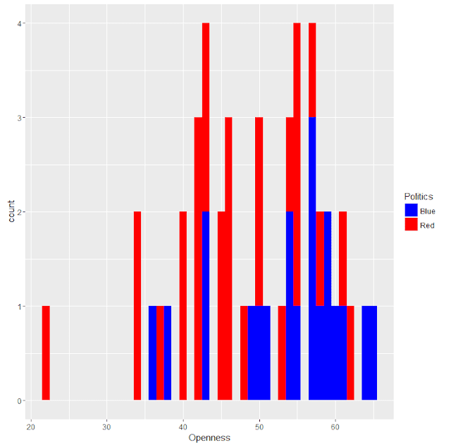
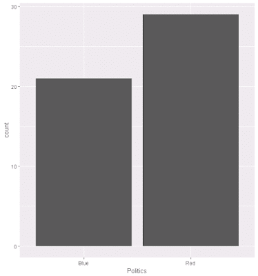
This is an example of Support Vector Machines, using one of my usual data sets, as part of a Pluralsight training presentation, Data Mining Algorithms in SSAS, Excel, and R . In terms of results, the prediction primarily predicts voter leanings based on two (2) traits, openness and conscientiousness, and although using all five (5) factors improved the prediction quality, plotting that is problematic. For this, the model is 96% predictive of Republican outcomes, but only 66% accurate in predicting Democratic leaning. Politics.prediction Blue Red Blue 15 1 Red 5 27 The code is below, as are some related graphs. Source data is here . # Clear memory rm(list = ls()) # set Working directory getwd() setwd('../Data') # load data Politics.df <- read.csv("BigFiveScoresByState.csv", na.strings = c("", "NA")) # clean data - remove NULLs Politics.df <- na.omit(Politic...

Decision Trees (party) on Political Outcome Based on State-level Big Five Assessment

Image
This decision tree demo is similar to a prior one I've done, but in this case, it uses the party package, that produces much higher-quality graphics than rpart, at least when used with plot. Although the idea for this analysis is mine, this was done as part of work for a Pluralsight training presentation, Data Mining Algorithms in SSAS, Excel, and R . Source data is here . # # Load Data # # Set working directory setwd("../Data") getwd() # read from data frame BigFivByState.df <- read.table("BigFiveScoresByState.csv", header = TRUE, sep = ",") # # Run Analysis # # Load package, install.packages('party', dependencies = TRUE) library(party) # train the model BigFivByState.dt <- ctree(data = BigFivByState.df, Liberal ~ Openness + Conscientiousness + Extraversion + Neuroticism + Agreeableness) # plot result plot(BigFivByState.dt, uniform = TRUE, main = ...

Naive Bayes on Political Outcome Based on State-level Big Five Assessment

Image
As part of another Pluralsight training presentation, Data Mining Algorithms in SSAS, Excel, and R , I worked through various exercises, and from that I've adapated Naive Basyes to one of my existing data sets. The code is below, as are some related graphs. Overall, the percent correct predicted based on Big Five personality traits using the Naive Bayes calculation is 66%. Source data is here . # # Load & Explore Data # # read from data frame BigFivByState.df <- read.table("BigFiveScoresByState.csv", header = TRUE, sep = ",") # review data head(BigFivByState.df) nrow(BigFivByState.df) summary(BigFivByState.df) names(BigFivByState.df) # various aggregations # as "count this value" ~ grouped by this + this Liberal.dist <- aggregate(State ~ Liberal, data = BigFivByState.df, FUN = length) head(Liberal.dist) RedBlue.dist <- aggregate(State ~ Politics, data = BigFivByState.df, FU...

Decision Tree in R, with Graphs: Predicting State Politics from Big Five Traits

Image
This was a continuation of prior explorations, logistic regression predicting Red/Blue state dichotomy by income or by personality. This uses the same five personality dimensions, but instead builds a decision tree. Of the Big Five traits, only two were found to useful in the decision tree, conscientiousness and openness. Links to sample data, as well as to source references, are at the end of this entry. Example Code # Decision Tree - Big Five and Politics library("rpart") # grow tree input.dat <- read.table("BigFiveScoresByState.csv", header = TRUE, sep = ",") fit <- rpart(Liberal ~ Openness + Conscientiousness + Neuroticism + Extraversion + Agreeableness, data = input.dat, method="poisson") # display the results printcp(fit) # visualize cross-validation results plotcp(fit) # detailed summary of splits summary(fit) # plot tree plot(fit, uniform = TRUE, main = "Class...

Chi-Square in R on by State Politics (Red/Blue) and Income (Higher/Lower)

This is a significant result, but instead of a logistic regression looking at the income average per state and the likelihood of being a Democratic state, it uses Chi-Square. Interpreting this is pretty straightforward, in that liberal states typically have cities and people that earn more money. When using adjusted incomes, by cost of living, this difference disappears. Example Code # R - Chi Square rm(list = ls()) stateData <- read.table("CostByStateAndSalary.csv", header = TRUE, sep = ",") # Create vectors affluence.median <- median(stateData$Y2014, na.rm = TRUE) affluence.v <- ifelse(stateData$Y2014 > affluence.median, 1, 0) liberal.v <- stateData$Liberal # Solve pol.Data = table(liberal.v, affluence.v) result <- chisq.test(pol.Data) print(result) print(pol.Data) Example Results Pearson's Chi-squared test with Yates' continuity correction data: pol.Data X-squared = 12.672, ...

Logistic Regression in R on State Voting in National Elections and Income

This data set - a link is at the bottom - is slightly different, income by state and political group, red or blue. Generally, residents of blue states have higher incomes, although not when adjusted for cost of living: Example Code # R - Logistic Regression stateData <- read.table("CostByStateAndSalary.csv", header = TRUE, sep = ",") am.data = glm(formula = Liberal ~ Y2014, data = stateData, family = binomial) print(summary(am.data)) Example Results Call: glm(formula = Liberal ~ Y2014, family = binomial, data = stateData) Deviance Residuals: Min 1Q Median 3Q Max -2.4347 -0.7297 -0.4880 0.6327 1.8722 Coefficients: Estimate Std. Error z value Pr(>|z|) (Intercept) -9.325e+00 2.671e+00 -3.491 0.000481 *** Y2014 1.752e-04 5.208e-05 3.365 0.000765 *** --- Signif. codes: 0 ‘***’ 0.001 ‘**’ 0.01 ‘*’ 0.05 ‘.’ 0.1 ‘ ’ 1 (Dispersion parameter for...