Data Analytics Workouts

Photo by Viktoria Alipatova from Pexels Responding to a Treehugger article, Why Americans will never love tea as much as coffee , I initially wrote my personal preferences for tea and coffee , ending with, BTW, this has just given me an idea for comparing Hofstede's cultural dimensions and coffee and tea consumption. Afterward, I did some analysis in Excel, then ran the same processes in R using Visual Studio, then converted that to a Jupyter Notebook on Microsoft's Azure Notebooks . Although this analysis is limited to 45 countries that have Hofstede's Cultural Dimensions , as well as per capita consumption for both coffee and tea, it would seem that coffee consumption correlates with power distance, individuality, and masculinity. Tea had small correlations with the dimensions and sometimes in the same direction as coffee. A fuller analysis is available on Microsoft's Azure Notebook , but some quick findings: Higher power distance, lower coffee consumption...

As part of my self-development, I wanted to rework a script, which are typically one-offs, and turn it into a reusable component, although there are existing packages for VaR. As such, this is currently a work in progress. This code is a Python-based class for VaR calculations , and for those unfamiliar with VaR, it is an acronym for value at risk, the worst case loss in a period for a particular probability. It is a reworking of prior work with scripted VaR calculations , implementing various high-level good practices, e.g., hiding/encapsulation, do-not-repeat-yourself (DRY), dependency injection, etc. Features: Requires data frame of stock returns, factor returns, and stock weights Expose a method to calculate and return a single VaR number for different variance types Expose a method to calculate and return an array of VaR values by confidence level Expose a method to calculate and plot an array of VaR values by confidence level Still to do: Dynamic factor usage Note...

The following modules linked below are based on a Pluralsight course, Understanding and Applying Financial Risk Modeling Techniques , and while the code itself is nearly verbatim, this is mostly for my own development, working through the peculiarities of Value at Risk (VaR) in both R and Python, and adding commentary as needed. The general outline of this process is as follows: Load and clean Data Calculate returns Calculate historical variance Calculate systemic, idiosyncratic, and total variance Develop a range of stress variants, e.g. scenario-based possibilities Calculate VaR as the worst case loss in a period for a particular probability The modules: In R: Financial Risk - Calculating Value At Risk (VaR) with R In Python: Financial Risk - Calculating Value At Risk (VaR) with Python

ARIMA is an acronym for Autoregressive Integrated Moving Average, and one explanation describes ARIMA models as... ...another approach to time series forecasting. Exponential smoothing and ARIMA models are the two most widely-used approaches to time series forecasting, and provide complementary approaches to the problem. While exponential smoothing models were based on a description of trend and seasonality in the data, ARIMA models aim to describe the autocorrelations in the data. A detailed technical discussion can be found on Wikipedia. For the first exploration I developed several ARIMA models using financial data, varying the parameters, noted as P, D and Q. A general overview of the parameters is from Wikipedia: p is the order (number of time lags) of the autoregressive model d is the degree of differencing (the number of times the data have had past values subtracted) q is the order of the moving-average model # filtered to start on a date Portfolio.filtere...

This is an example of neural networks using the neuralnet package on one of my sample data sets, walking through a Pluralsight training series, Data Mining Algorithms in SSAS, Excel, and R . In terms of results, the regression primarily predicts voter leanings based on five (5) traits, openness, conscientiousness, extraversion, agreeableness, and neuroticism, although only the first two (2) traits have a significant impact. Logistic regression is about 85% predictive, and slightly better at predicting Red states over its ability in predicting Blue states. [1] "Logistic Regression (All) - Correct (%) = 0.854166666666667" [1] "Logistic Regression (Red) - Correct (%) = 0.892857142857143" [1] "Logistic Regression (Blue) - Correct (%) = 0.8" For the neuralnet package, I created a loop to vary the hidden layers and the number of repetitions, since this is such a small number of records. This is obviously much less predictive than logistic regressi...

As part of a Pluralsight training presentation, Understanding and Applying Logistic Regression , students worked through various exercises, one of which was predicting stock price changes, up or down, on Google, using Google and Spyder closing prices. As an ordered list of actions: Load data - Yahoo financials for each day for 5 years, taking only date and closing price for this analysis Transform sources: Merge sources, change column headings, cast the Date column as DATE type, sort descending Perform logistic regression Create a frame of actual versus predicted changes, and add a column for the correct/incorrect prediction result Find percent correct, on whether the price moved correctly up or down As a result, the lagged Google and SPY prices accurately predict next day prices about 63% of the time. Source data is here . # Clear memory rm(list = ls()) # Set working directory setwd("../Data") getwd() # load data # Data is Yahoo finan...

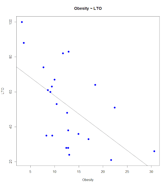
Hofstede extended his original four dimensions, adding measures Long-Term Orientation (LTO) and Indulgence (Ind) in response to other researchers studies. While reading Hofstede's Cultures and Organizations: Software of the Mind, Third Edition I was struck by the lackluster reporting of the correlation between obesity and indulgence. It seemed obvious one would delve a bit further, maybe looking at a compound relationship between both indulgence and LTO, e.g., does short-sightedness and indulgence lead to obesity. Although I limit my analysis to OECD countries, that is what I present here. An explanation of dimensions can be found on Hofstede's site. Hofstede's Dimensions and Obesity A first step would be to see what relationships exist between obesity and the dimensions: 1: # LM - Multiple Regression - New Hofstede, LTO and Ind 2: # Load the data into a matrix 3: rm(list = ls()) 4: setwd("../Data") 5: oecdData <- read.table("OECD ...