Data Analytics Workouts

This article in the NY Times is to some degree an example of the problem of survivor bias, or generalizing from the few successful individuals to all individuals Do Olympians Get Too Much Exercise? My comment: One obvious problem with this type of study, is that athletes that might have developed issues might no longer engage in, and might have previously given up, said activities. If you only look at the winners, and not the losers, one gets an unfair picture of the effect or traits on all participants. Yes, you know that the winners did not have problems, but what about those that gave the activity up, or died?

An article, Fifty States of Anxiety in the NY Times annoyed me a bit, and it highlighted what happens when people do not look at all the relevant variables. It also seems that the author seems to have expressed his opinion in a way that was not supported by the data. The fact that his analysis did not match his data indicates his bias. My comment: As I mentioned in another post, there are regional differences in personality, and if you only know anxiety and red-state blue dichotomies the map makes no sense. What you need are 3 dimensions of the Big Five personality inventory, openness to experience, neuroticism, and conscientiousness. Also, you need to know that the strongest predictor of liberal leaning is openness, while there is also a slight correlation with conscientiousness and conservatism. Neuroticism has no relationship with political orientation. When one realizes that the strong openness areas are the Pacific and NorthEast regions, and the strong conscientiousness region

A interesting article by six statisticians, Ten Simple Rules for Effective Statistical Practice . Their aim: To this point, Meng notes "sound statistical practices require a bit of science, engineering, and arts, and hence some general guidelines for helping practitioners to develop statistical insights and acumen are in order. No rules, simple or not, can be 100% applicable or foolproof, but that's the very essence that I find this is a useful exercise. It reminds practitioners that good statistical practices require far more than running software or an algorithm." The 10 rules are: Statistical Methods Should Enable Data to Answer Scientific Questions Signals Always Come with Noise Plan Ahead, Really Ahead Worry about Data Quality Statistical Analysis Is More Than a Set of Computations Keep it Simple Provide Assessments of Variability Check Your Assumptions When Possible, Replicate! Make Your Analysis Reproducible

Responses to a post on the correlation between country-average IQ and responding yes to a question on if religion matters are inversely correlated, but not strongly so, prompted me to dig up a more significant issue, the relationship between religiosity and inequality, as measured by the Gini coefficient. The correlation is quite high, at about .7, although this really says nothing about the cause, if religious countries tend toward inequality because of general tendencies, or if inequality drives people to religion, as a salve against suffering. In truth, they could both be reflective of some other aspect of a country, and not in any way causative. Example Code # Correlations on ReligionMatters and Gini Coeficients oecdData <- read.table("OECD - Quality of Life.csv", header = TRUE, sep = ",") #names(oecdData) religionMattersVector <- oecdData$ReligionMatters giniVector <- oecdData$Gini cor.test(giniVector, religionMattersVect

I was reminded this morning by an article, New Study: Religious People Are Less Smart but Atheists Are Psychopaths . but realized that there are many studies showing the religious to be less intelligent, but rarely is this ever published. It would 'bite' most of the population, liberal and conservative alike. Note : I plan on redoing this with more solid numbers, and possibly different measures of religiosity. Example Code # Correlations on ReligionMatters and Average IQ oecdData <- read.table("OECD - Quality of Life.csv", header = TRUE, sep = ",") iqVector <- oecdData$IQ religionMattersVector <- oecdData$ReligionMatters cor.test(iqVector, religionMattersVector) lm1 <- lm(iqVector ~ religionMattersVector) summary(lm1) # Plot the chart. plot(iqVector, religionMattersVector, col = "blue", main = "IQ ~ Religion Matters Vector" , abline(lm(religionMattersVector ~ iqVector),

This was a continuation of prior explorations, logistic regression predicting Red/Blue state dichotomy by income or by personality. This uses the same five personality dimensions, but instead builds a decision tree. Of the Big Five traits, only two were found to useful in the decision tree, conscientiousness and openness. Links to sample data, as well as to source references, are at the end of this entry. Example Code # Decision Tree - Big Five and Politics library("rpart") # grow tree input.dat <- read.table("BigFiveScoresByState.csv", header = TRUE, sep = ",") fit <- rpart(Liberal ~ Openness + Conscientiousness + Neuroticism + Extraversion + Agreeableness, data = input.dat, method="poisson") # display the results printcp(fit) # visualize cross-validation results plotcp(fit) # detailed summary of splits summary(fit) # plot tree plot(fit, uniform = TRUE, main = "Class

This was a little bit of fun, after reading a few more chapters of Text Analysis with R for Students of Literature . Spinoza is a current interest, as I am also reading Radical Enlightenment: Philosophy and the Making of Modernity 1650-1750 . Example Code (Common to Subsections) # Text for this can be acquired as below Project Gutenberg, as below # http://www.gutenberg.org/cache/epub/989/pg989.txt, # or via a Sample Data at the end of this post: textToRead = 'pg989.txt' # Text for this can be acquired via Matthew Jockers site, as below, # http://www.matthewjockers.net/macroanalysisbook/expanded-stopwords-list/, # or via a Sample Data at the end of this post: exclusionFile = 'StopList_Extended.csv' # Read Text text.scan <- scan(file = textToRead, what = 'char') text.scan <- tolower(text.scan) # Create list text.list <- strsplit(text.scan, '\\W+', perl = TRUE) text.vector <- unlist(text.list) # Create

As part of the Data science is OSEMN module for Obtaining Data I worked through the exercises. Example Code # Exercises """http://people.duke.edu/~ccc14/sta-663/DataProcessingSolutions.html#exercises""" """1. Write the following sentences to a file “hello.txt” using open and write. There should be 3 lines in the resulting file. Hello, world. Goodbye, cruel world. The world is your oyster.""" str = 'Data\Test.txt' f = open(str, 'w') f.write('Hello, world.\r') f.write('Goodbye, cruel world.\r') f.write('The world is your oyster.') # Writes same thing, only in one statement f.write('\rHello, world.\rGoodbye, cruel world.\rThe world is your oyster.') f.close() with open(str, 'r') as f: content = f.read() print(content) """2. Using a for loop and open, print o

OESMN is an acronym, for the elements of data science: Obtaining data Scrubbing data Exploring data Modeling data iNterpreting data As part of the Data science is OSEMN module  for Obtaining Data I performed the examples myself, as well as with variants. Example Code # Data science is OSEMN """http://people.duke.edu/~ccc14/sta-663/DataProcessingSolutions.html#data-science-is-osemn""" # Acquiring data """Plain text files We can open plain text files with the open function. This is a common and very flexible format, but because no structure is involved, custom processing methods to extract the information needed may be necessary. Example 1: Suppose we want to find out how often the words alice and drink occur in the same sentence in Alice in Wonderland. This example uses Gutenberg: http://www.gutenberg.org/wiki/Main_Page, a good source for files""" # the data file is linked below

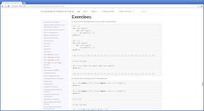
I worked through Exercises section of the Computational Statistics in Python tutorial . Below are the results, with some variations i generated to get a better understanding of the solutions: # Exercises """http://people.duke.edu/~ccc14/sta-663/FunctionsSolutions.html#exercises""" """1. Rewrite the following nested loop as a list comprehension ans = [] for i in range(3): for j in range(4): ans.append((i, j)) print ans""" arr = [(i,j) for i in range(3) for j in range(4)] arr """2. Rewrite the following as a list comprehension ans = map(lambda x: x*x, filter(lambda x: x%2 == 0, range(5))) print ans""" arr = [x**2 for x in range(5) if x%2 == 0] """3. Convert the function below into a pure function with no global variables or side effects x = 5 def f(alist): for i in r

I worked through functools and itertools sections of the Computational Statistics in Python tutorial , and I found these promisingly powerfuul for data modeling and functional programming: # The functools module """The most useful function in the functools module is partial, which allows you to create a new function from an old one with some arguments “filled-in”.""" from functools import partial def power_function(power, num): """power of num.""" return num**power square = partial(power_function, 2) cube = partial(power_function, 3) quad = partial(power_function, 4) # The itertools module """This provides many essential functions for working with iterators. The permuations and combinations generators may be particularly useful for simulations, and the groupby gnerator is useful for data analyiss.""" from itertools import cyc

I worked through Iterators, Generators and Decorators sections of the Computational Statistics in Python tutorial , and although this code is similar to the tutorial, it is modified in ways to make it retainable to myself: # Iterators can be created from sequences with the built-in function iter() """http://people.duke.edu/~ccc14/sta-663/FunctionsSolutions.html#iterators""" xs = [n for n in range(10)] x_iter = iter(xs) [x for x in x_iter] for x in x_iter: print(x) # Generators """http://people.duke.edu/~ccc14/sta-663/FunctionsSolutions.html#generators""" # Functions containing the 'yield' keyword return iterators # After yielding, the function retains its previous state def limit_seats(n): """Limits number and counts down""" for i in range(n, 0, -1): yield i counter = limit_seats(10) for count in

I worked through recursion in the Computational Statistics in Python tutorial , getting up to speed on Python, and although this code is similar to the tutorial, I did try to 'make it mine': # Recursion """http://people.duke.edu/~ccc14/sta-663/FunctionsSolutions.html#recursion""" # Correct Example def fibonacci(n): if n==0 or n==1: return 1 else: return fibonacci(n-1) + fibonacci (n-2) [fibonacci(n) for n in range(10)] def fibonacciWithCache(n, cache={0:1, 1:1}): try: return cache[n] except: cache[n] = fibonacci(n-1) + fibonacci (n-2) return cache[n] [fibonacciWithCache(n) for n in range(10)] # Correct Example def factorial(n): if n==0: return 1 else: return n * factorial(n-1) # Correct Example, with caching def factorialWithCache(n, cache={0:1}): try: return cache[n] except KeyError: cache[

I am currently working through Computational Statistics in Python 's module Functions are first class objects , and for this - I have worked with delegates and higher order functions in other languages - I put together this example to better grasp higher order functions in Python: def power_function(num, power): """power of num.""" return num**power def add_function(num, more): """sum of num.""" return num+more def runFunction(fx, x, y): return fx(x,y) num = 2 powers = range(0,64) arrPower = list(map(lambda x: runFunction(power_function, num, x), powers)) arrAdd = list(map(lambda x: runFunction(add_function, num, x), powers)) arrPower arrAdd

To prepare for further exploration in data analytics, and give myself some time to absorb R, I decided to work in Python for a while. For this, I worked through Computational Statistics in Python module Introduction to Python . These are some of the code produced to solve the exercises: # Tutorial Answers """http://people.duke.edu/~ccc14/sta-663/IntroductionToPythonSolutions.html""" """1. Solve the FizzBuzz problem “Write a program that prints the numbers from 1 to 100. But for multiples of three print “Fizz” instead of the number and for the multiples of five print “Buzz”. For numbers which are multiples of both three and five print “FizzBuzz”.""" def fizz_buzz(begin, end): """Write a program that prints the numbers from 1 to 100. But for multiples of three print “Fizz” instead of the number and for the multiples of five print “Buzz”. For numbers which are multi

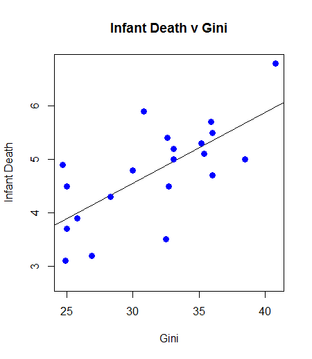
At a correlation approaching 0.7, the relationship between infant mortality and inequality is quite high. One can argue causality, but the existence of the relationship, and there are others of varying magnitude, is a powerful indictment: Example Code oecdData <- read.table("OECD - Quality of Life.csv", header = TRUE, sep = ",") gini.v <- oecdData$Gini death.v <- oecdData$InfantDeath cor.test(gini.v, death.v) plot(gini.v, death.v, col = "blue", main = "Infant Death v Gini" , abline(lm(death.v ~ gini.v)) , cex = 1.3, pch = 16, xlab = "Gini", ylab = "Infant Death") Example Results Pearson's product-moment correlation data: gini.v and death.v t = 4.2442, df = 19, p-value = 0.0004387 alternative hypothesis: true correlation is not equal to 0 95 percent confidence interval: 0.3805316 0.8679275 sample estimates: cor 0.69762 Example Graph Sample

These are rudimentary functions created in Python, working through the exercises in Computational Statistics in Python from Duke . def power_function(num, power): """Funcion to caculate power, number ** power.""" return num**power def fizz_buzz(begin, end): """Write a program that prints the numbers from 1 to 100. But for multiples of three print “Fizz” instead of the number and for the multiples of five print “Buzz”. For numbers which are multiples of both three and five print “FizzBuzz""" for i in range(begin, end): if i%3 == 0 & i%5 == 0: print("FizzBuzz") elif i%5 == 0: print("Buzz") elif i%3 == 0: print("Fizz") else: print(1) def euclidean(UPoint, VPoint, ShortCalc): """Write a function that calculates and returns the euclidean distance between two

I was working through a tutorial in Python, but found this one, Computational Statistics in Python from Duke , much better. It has exercises, which increase retention, and the material is well-presented.

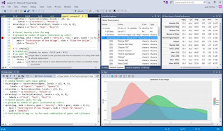
I recently finished a tutorial I was working through in R - I have certainly not exhausted exploring R, just taking time to let it settle in - and am thinking of working with Python for a while. That would include using  Python Tools for Visual Studio :

This is a significant result, but instead of a logistic regression looking at the income average per state and the likelihood of being a Democratic state, it uses Chi-Square. Interpreting this is pretty straightforward, in that liberal states typically have cities and people that earn more money. When using adjusted incomes, by cost of living, this difference disappears. Example Code # R - Chi Square rm(list = ls()) stateData <- read.table("CostByStateAndSalary.csv", header = TRUE, sep = ",") # Create vectors affluence.median <- median(stateData$Y2014, na.rm = TRUE) affluence.v <- ifelse(stateData$Y2014 > affluence.median, 1, 0) liberal.v <- stateData$Liberal # Solve pol.Data = table(liberal.v, affluence.v) result <- chisq.test(pol.Data) print(result) print(pol.Data) Example Results Pearson's Chi-squared test with Yates' continuity correction data: pol.Data X-squared = 12.672,

This data set - a link is at the bottom - is slightly different, income by state and political group, red or blue. Generally, residents of blue states have higher incomes, although not when adjusted for cost of living: Example Code # R - Logistic Regression stateData <- read.table("CostByStateAndSalary.csv", header = TRUE, sep = ",") am.data = glm(formula = Liberal ~ Y2014, data = stateData, family = binomial) print(summary(am.data)) Example Results Call: glm(formula = Liberal ~ Y2014, family = binomial, data = stateData) Deviance Residuals: Min 1Q Median 3Q Max -2.4347 -0.7297 -0.4880 0.6327 1.8722 Coefficients: Estimate Std. Error z value Pr(>|z|) (Intercept) -9.325e+00 2.671e+00 -3.491 0.000481 *** Y2014 1.752e-04 5.208e-05 3.365 0.000765 *** --- Signif. codes: 0 ‘***’ 0.001 ‘**’ 0.01 ‘*’ 0.05 ‘.’ 0.1 ‘ ’ 1 (Dispersion parameter for

Similar to the post about linear regression, Linear Regression with R, on IQ for Gini and Linguistc Diversity , this the same data used for multiple regression, with some minor but statistically significant examples: Example Code # LM - Multiple Regression # Load the data into a matrix oecdData <- read.table("OECD - Quality of Life.csv", header = TRUE, sep = ",") print(names(oecdData)) # Access the vectors v1 <- oecdData$IQ v2 <- oecdData$HofstederPowerDx v3 <- oecdData$HofstederMasculinity v4 <- oecdData$HofstederIndividuality v5 <- oecdData$HofstederUncertaintyAvoidance v6 <- oecdData$Diversity_Ethnic v7 <- oecdData$Diversity_Linguistic v8 <- oecdData$Diversity_Religious v9 <- oecdData$Gini # Gini ~ Hofstede relation1 <- lm(v9 ~ v2 + v3 + v4 + v5) print(relation1) print(summary(relation1)) print(anova(relation1)) # IQ ~ Hofstede Individuality, Linguistic Diversity

Reusing the code posted for Correlations within with Hofstede's Cultural Values, Diversity, GINI, and IQ , the same data can be used for linear regression: Example Code # LM - Linear Regression # Load the data into a matrix oecdData <- read.table("OECD - Quality of Life.csv", header = TRUE, sep = ",") # Access the vectors v1 <- oecdData$IQ v2 <- oecdData$HofstederPowerDx v3 <- oecdData$HofstederMasculinity v4 <- oecdData$HofstederIndividuality v5 <- oecdData$HofstederUncertaintyAvoidance v6 <- oecdData$Diversity_Ethnic v7 <- oecdData$Diversity_Linguistic v8 <- oecdData$Diversity_Religious v9 <- oecdData$Gini # IQ ~ Gini relation1 <- lm(v1 ~ v9) print(relation1) print(summary(relation1)) # IQ ~ Diversity_Linguistic relation2 <- lm(v1 ~ v7) print(relation2) print(summary(relation2)) Example Results > # Access the vectors + v1 <- oecdData$IQ

Reusing the code posted for Correlations within with Hofstede's Cultural Values, Diversity, GINI, and IQ , the same data can be used for mean, median, and mode. Additionally, the summary function will return values in addition to mean and median, Min, Max, and quartile values: Example Code oecdData <- read.table("OECD - Quality of Life.csv", header = TRUE, sep = ",") v1 <- oecdData$IQ # Mean with na.rm = TRUE removed NULL avalues mean(v1, na.rm = TRUE) # Median with na.rm = TRUE removed NULL values median(v1, na.rm = TRUE) # Returns the same data as mean and median, but also includes distribution values: # Min, Quartiles, and Max summary(v1) # Mode does not exist in R, so we need to create a function getmode <- function(v) { uniqv <- unique(v) uniqv[which.max(tabulate(match(v, uniqv)))] } #returns the mode getmode(v1) Example Results > oecdData <- read.table("OECD - Quality

Similar to the code I posted for ANOVA with Hofstede's Cultural Values and Economic Outcomes , you can perform correlations on the same data, for the same countries and for the similar vectors. The data file is linked via Google Drive at the end of this post. Countries [1] Australia Austria Belgium Canada Denmark [6] Finland France Germany Greece Iceland [11] Ireland Italy Japan Korea Luxembourg [16] Netherlands New Zealand Norway Portugal Spain [21] Sweden Switzerland United Kingdom United States Data Columns [1] "Country" "HofstederPowerDx" [3] "HofstederIndividuality" "HofstederMasculinity" [5] "HofstederUncertaintyAvoidance" "Diversity_Ethnic" [7] "Diversity_Linguistic" &qu

While in B-School, back around 2002, I considered trying to get published, partially because I had done well enough in economics and finance - A's in everything, and disturbed the curve in Financial Economics - to be a member of the International Economics Honor Society, which came with a subscription to American Economics, and that came with an opportunity to publish. Nothing came of it, other than highly illuminating correlations between income inequality (Gini Coefficient) and negative social outcomes, but I kept the data, and can now use it with R. To make the data more relevant to ongoing political discourse, it was limited to developed countries in the OECD. The data file is linked via Google Drive at the end of this post. Countries [1] Australia Austria Belgium Canada Denmark [6] Finland France Germany Greece Iceland [11] Ireland Italy Japan Korea Luxembourg [16]

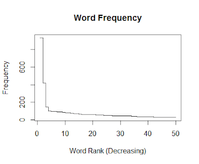
I spent a little time trying to find a simple parser for text files, and this certainly works, and is straightforward: Example Code # Simple word frequency # # Read text wordCount.text <- scan(file = choose.files(), what = 'char', sep = '\n') # Removes whitepace wordCount.text <- paste(wordCount.text, collapse = " ") # Convert to lower wordCount.text <- tolower(wordCount.text) # Split on white space wordCount.words.list <- strsplit(wordCount.text, '\\W+', perl = TRUE) # convert to vector wordCount.words.vector <- unlist(wordCount.words.list) # table method builds word count list wordCount.freq.list <- table(wordCount.words.vector) # Sorts word count list wordCount.sorted.freq.list <- sort(wordCount.freq.list, decreasing = TRUE) # Concantenates the word and count before export wordCount.sorted.table <- paste(names(wordCount.sorted.freq.list), wordCount.sorted

As part of getting up to speed, I reworked some basic code I created for solver Project Euler problems using F# into R: # Fibonacci series # fibsRec <- function(a, b, max, arr) { if (a + b > max) { arr } else { current = a + b newArr = arr newArr[length(arr)+1] = current fibsRec(b, current, max, newArr) } } startList <- c(1,2) result <- fibsRec(1, 2, 40, startList) print(result) # Project Euler - Problem #1 # # Find a way of finding the sum of all the multiples of 3 or 5 below 1000 # if we list all the natural numbers below 10 that are multiples of 3 or 5, # we get 3, 5, 6 and 9. The sum of these multiples is 23. # Find the sum of all the multiples of 3 or 5 below 1000. # rm(list = ls()) num <- seq(1:999) filteredList <- function(l) { newArr <- c(0) for (i in l) { if (i %% 3 == 0 || i %% 5 == 0) {

Macroanalysis by Matthew L. Jockers My rating: 4 of 5 stars Great foray into data mining literature, although at times a bit tedious and redundant. Conceptually useful, for general concepts in data mining, but with no actual coding. View all my reviews

After Microsoft's announcement,  Announcing R Tools for Visual Studio | Machine Learning Blog , I downloaded R Tools and R Open 3.2.3, and have now begin working through tutorials, the first being Tutorials Point's R Tutorial . Much of the syntax would be common to any programmer, and some of the conventions are common in languages like F#, which is use lists and array extensively, with a similar style for assignment.

While searching for a primer on how to use R in Visual Studio, I ran across this: An infographic Choosing R or Python for data analysis? An infographic

Although I have always had an interest in data and analytics, Microsoft's recent moves to incorporate R into SQL Server, as well as Visual Studio's integration with Python, makes learning data analytics an easier option, as well as a likely necessity for my career. It is not that I would not enjoy analysis on my own: I was likely the only person really capable of writing SAS in my Statistics for the Social Sciences, and ran so many correlations for my study on education and fitness I was almost banned from the lab While in B-school, around 2002, I looked to analyze and publish the relationship between Hofstede's cultural dimensions and OECD economic data Eventually, I found significant negative relationships between income inequality on social welfare, years before it became widely popularized