Neural Networks in R (Part 3 of 4) - Neural Networks on Price Changes in Financial Data
This post is a demonstration using the caret and nnet packages on aggregate Big Five traits per state and political leanings, and a continuation of a series:
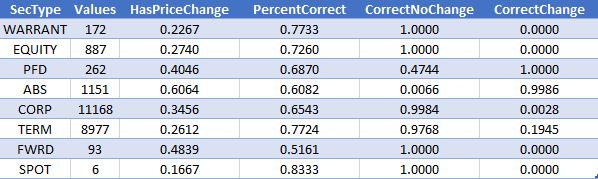
Initially, the results seemed promising, with a prediction accuracy of ~.85, further analysis revealed that the bulk of accurate predictions were those that had no price change, and that price change classes were often inaccurate. I excluded security types without price change, and the average dropped even further. I then created a loop that calculated test and training data by security type, and those result indicated that the neural net very right and very wrong, for price change state. Only one security seemed remotely predicted, that of PFD.
The code is below, as are some related graphs. Source data cannot be provided.
- Neural Networks (Part 1 of 4) - Logistic Regression and neuralnet on State 'Personality' and Political Outcomes
- Neural Networks (Part 2 of 4) - caret and nnet on State 'Personality' and Political Outcomes
Initially, the results seemed promising, with a prediction accuracy of ~.85, further analysis revealed that the bulk of accurate predictions were those that had no price change, and that price change classes were often inaccurate. I excluded security types without price change, and the average dropped even further. I then created a loop that calculated test and training data by security type, and those result indicated that the neural net very right and very wrong, for price change state. Only one security seemed remotely predicted, that of PFD.

The code is below, as are some related graphs. Source data cannot be provided.
 ################################################
 # create formula used for all samples
 ################################################

 #names(Portfolio.df)
 equation <- as.formula("PriceChange ~ Coupon + Duration + Convexity")


 ################################################3
 # Neural Net with nnet and caret
 # Filtering comparisons
 ################################################3

 # load packages
 library(nnet)
 library(caret)

 # set parameters for loop
 secTypes <- unique(Portfolio.df$Sec_Type)
 numRows <- length(secTypes)

 # create empty data frame, for best performance
 Filtered.Predictions <- data.frame(SecType = character(numRows), Values = numeric(numRows), HasPriceChange = numeric(numRows), PercentCorrect = numeric(numRows), PercentCorrectNoChange = numeric(numRows), PercentCorrectChange = numeric(numRows), stringsAsFactors = FALSE)

 # loop through parameters and neural net to buil;d results
 currentRow = 0
 for (secType in secTypes) {

   currentRow <- currentRow + 1

   # filter data set
   Portfolio.filtered <- Portfolio.df.preclean[Portfolio.df.preclean$Sec_Type == secType,]
   #View(Portfolio.df.preclean)

   # only work on assets with price changes
   if ((sum(ifelse(Portfolio.filtered$PriceChange == 1, 1, 0)) / nrow(Portfolio.filtered)) >= 0.0) {

     # add sec type to result data frame
     Filtered.Predictions$SecType[currentRow] <- secType

     # add number of values to result data frame
     Filtered.Predictions$Values[currentRow] <- nrow(Portfolio.filtered)
     Filtered.Predictions$HasPriceChange[currentRow] <- (sum(ifelse(Portfolio.filtered$PriceChange == 1, 1, 0)) / nrow(Portfolio.filtered))

     # train
     Portfolio.filtered.train <- train(equation, Portfolio.filtered, method = 'nnet', linout = TRUE, trace = FALSE)

     # predict
     Portfolio.filtered.predicted <- predict(Portfolio.filtered.train, Portfolio.filtered)

     # combine
     Portfolio.filtered.combined <- cbind(Portfolio.filtered.predicted, Portfolio.filtered)

     # calculate correct
     Portfolio.filtered.combined$predictionBinary <- ifelse(Portfolio.filtered.combined$Portfolio.filtered.predicted >= .5, 1, 0)
     Portfolio.filtered.combined$Correct <- ifelse(Portfolio.filtered.combined$predictionBinary == Portfolio.filtered.combined$PriceChange, 1, 0)
     correct <- (sum(Portfolio.filtered.combined$Correct) / length(Portfolio.filtered.combined$Correct))

     # calculate correct, no change
     Portfolio.filtered.combined.NoChange <- Portfolio.filtered.combined[Portfolio.filtered.combined$PriceChange == 0,]
     correctNoChange <- (sum(Portfolio.filtered.combined.NoChange$Correct) / length(Portfolio.filtered.combined.NoChange$Correct))

     # calculate correct, change
     Portfolio.filtered.combined.Change <- Portfolio.filtered.combined[Portfolio.filtered.combined$PriceChange == 1,]
     correctChange <- (sum(Portfolio.filtered.combined.Change$Correct) / length(Portfolio.filtered.combined.Change$Correct))

     # add percent correct to result
     Filtered.Predictions$PercentCorrect[currentRow] <- correct
     Filtered.Predictions$PercentCorrectNoChange[currentRow] <- correctNoChange
     Filtered.Predictions$PercentCorrectChange[currentRow] <- correctChange
   }
 }

 # display results
 Filtered.Predictions <- Filtered.Predictions[Filtered.Predictions$HasPriceChange > 0,]

 # plots percent correct for change versus percent correct for no change
 library(ggplot2)
 plotPart1 <- ggplot(data = Filtered.Predictions, aes(x = HasPriceChange, y = PercentCorrect))
 plotpart2 <- plotPart1 + geom_point() + stat_smooth(method = "lm", formula = y ~ x, size = 1)
 plotpart2 + geom_text(aes(label = SecType), hjust = 0, vjust = 0, nudge_x = -.00, nudge_y = .005, angle=0, size=3)


Comments
Post a Comment