Naive Bayes on Political Outcome Based on State-level Big Five Assessment

As part of another Pluralsight training presentation, Data Mining Algorithms in SSAS, Excel, and R, I worked through various exercises, and from that I've adapated Naive Basyes to one of my existing data sets.

The code is below, as are some related graphs. Overall, the percent correct predicted based on Big Five personality traits using the Naive Bayes calculation is 66%.

Source data is here.

 #   
 # Load & Explore Data  
 #  
   
 # read from data frame  
 BigFivByState.df <- read.table("BigFiveScoresByState.csv", header = TRUE, sep = ",")  
   
 # review data  
 head(BigFivByState.df)  
 nrow(BigFivByState.df)  
 summary(BigFivByState.df)  
 names(BigFivByState.df)  
   
 # various aggregations  
 # as "count this value" ~ grouped by this + this  
 Liberal.dist <- aggregate(State ~ Liberal, data = BigFivByState.df, FUN = length)  
 head(Liberal.dist)  
   
 RedBlue.dist <- aggregate(State ~ Politics, data = BigFivByState.df, FUN = length)  
 head(RedBlue.dist)  
   
 #   
 # plotting  
 #  
   
 # install ggplot  
 install.packages('ggplot2')  
 library(ggplot2)  
   
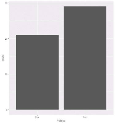
 # simple count per group  
 Political.dist <- ggplot(BigFivByState.df, aes(Politics), FUN = length)  
 Political.dist + geom_bar()  
 


 # charts with trendlines  
 cor.test(BigFivByState.df$Conscientiousness, BigFivByState.df$Openness)  
 OpennessVersusConscientiousness <- ggplot(BigFivByState.df, aes(x = Conscientiousness, y = Openness), FUN = length, na.rm = TRUE)  
 OpennessVersusConscientiousness + geom_line(na.rm = TRUE) + geom_smooth(method = lm, na.rm = TRUE)  
  
 cor.test(BigFivByState.df$Neuroticism, BigFivByState.df$Openness)  
 OpennessVersusNeuroticism <- ggplot(BigFivByState.df, aes(x = Neuroticism, y = Openness), FUN = length, na.rm = TRUE)  
 OpennessVersusNeuroticism + geom_line(na.rm = TRUE) + geom_smooth(method = lm, na.rm = TRUE)  
   
 cor.test(BigFivByState.df$Extraversion, BigFivByState.df$Neuroticism)  
 ExtraversionVersusNeuroticism <- ggplot(BigFivByState.df, aes(x = Neuroticism, y = Extraversion), FUN = length, na.rm = TRUE)  
 ExtraversionVersusNeuroticism + geom_line(na.rm = TRUE) + geom_smooth(method = lm, na.rm = TRUE)  
   
 cor.test(BigFivByState.df$Extraversion, BigFivByState.df$Openness)  
 ExtraversionVersusOpenness <- ggplot(BigFivByState.df, aes(x = Openness, y = Extraversion), FUN = length, na.rm = TRUE)  
 ExtraversionVersusOpenness + geom_line(na.rm = TRUE) + geom_smooth(method = lm, na.rm = TRUE)  
   
 


 #  
 # Naive Bayes  
 #  
   
 install.packages('e1071', dependencies = TRUE)  
 library(e1071)  
   
 # naive bayes  
 NaiveBayes <- naiveBayes(BigFivByState.df[, 2:11], BigFivByState.df$Politics)  
   
 # a priori probabilities for the target variables  
 NaiveBayes$apriori  
   
 # a priori probabilities for the input variables  
 NaiveBayes$tables  
   
 # data frame with predictions  
 predictions.df <- as.data.frame(predict(NaiveBayes, BigFivByState.df, type = 'raw'))  
  
  
 #   
 # Validate Results  
 #  
   
 # join predictions with source  
 predictions.joined <- cbind(BigFivByState.df, predictions.df)  
   
 # validate predictions  
 predictions.joined$Predicted <- ifelse(predictions.joined$Blue >= .05, "Blue", "Red")  
 predictions.joined$Check <- ifelse(predictions.joined$Politics == predictions.joined$Predicted, "Correct", "Incorrect")  
   
 # calculate right and wrong  
 length(predictions.joined$Check[predictions.joined$Check== "Correct"]) / length(predictions.joined$Check)  
   
 # chart count of right and wrong   
 ggplot(predictions.joined, aes(Check), FUN = length) + geom_bar()  
  


 # output  
 write.csv(predictions.joined, file = "JoinedPoliticaLPredictions.csv")