Data Analytics Workouts

I've been interested in Hofstede's work since B-school, back in the early second millennia, and at one time considered publishing using his country characteristics as predictors for economic and social welfare outcomes. Nowadays, I use the results of his analyses frequently in small R programming demonstrations. He's an interesting researcher, who's done important work, as The Economist article describes : The man who put corporate culture on the map—almost literally—Geert Hofstede (born 1928) defined culture along five different dimensions. Each of these he measured for a large number of countries, and then made cross-country comparisons. In the age of globalisation, these have been used extensively by managers trying to understand the differences between workforces in different environments. The Economist article give a fuller picture of Geert Hofstede , and anyone interested in reading one of his works might enjoy Cultures and Organizations: Software of the Mi...

I was exploring Jupyter notebooks , that combines live code, markdown and data, through Microsoft's implementation, known as MS Azure Notebooks , putting together a small library of R and F# notebooks . As Microsoft's FAQ for the service describes it as : ...a multi-lingual REPL on steroids. This is a free service that provides Jupyter notebooks along with supporting packages for R, Python and F# as a service. This means you can just login and get going since no installation/setup is necessary. Typical usage includes schools/instruction, giving webinars, learning languages, sharing ideas, etc. Feel free to clone and comment... In R Azure Workbook for R - Memoisation and Vectorization Charting Correlation Matrices in R In F# Charnownes Constant in FSharp.ipynb Project Euler - Problems 18 and 67 - FSharp using Dynamic Programming

Efficient R Programming: A Practical Guide to Smarter Programming by Colin Gillespie My rating: 5 of 5 stars Simply a great book, chock full of tips and techniques for improving one's work with R. View all my reviews

Full of potential coding improvements, Efficient R Programming: A Practical Guide to Smarter Programming , the book makes two suggestions that are notable. Vectorization, explained here and here , and memoisation , caching prior results albeit with additional memory use, were relevant and significant. What follows is a demonstration of the speed improvements that might be achieved using these concepts. ################################ # performance # vectorization and memoization ################################ # clear memory between changes rm(list = ls()) #load memoise #install.packages('memoise') library(memoise) # create test function monte_carlo = function(N) { hits = 0 for (i in seq_len(N)) { u1 = runif(1) u2 = runif(1) if (u1 ^ 2 > u2) hits = hits + 1 } return(hits / N) } # memoise test function monte_carlo_memo <- memoise(monte_carlo) # vectorize function monte_carlo...

While developing these demonstrations in logistic regression and neural networks, I used and discovered some interesting methods and techniques: Better Methods A few useful commands and packages...: update.packages() for updating installed packages in one easy action as.formula() for creating a formula that I can reuse and update in one action across all my code sections View() for looking at data frames fourfoldplot() for plotting confusion matrices neuralnet for developing neural networks caret , used with nnet , to create predictive model plotnet() in NeuralNetTools, for creating attractive neural network models Resources that I used or that I would like to explore... MS Azure Notebooks , for working online with Python, R, and F#, all part of MS's data workflows Efficient R Programming , that seems to have many good tips on working with R Data Mining Algorithms in SSAS, Excel, and R , showing various algorithms in each technology R Documentation , a ...

As part of writing analyses using neural networks I thought of displaying a confusion matrix, but went looking for something more. What I found was either ugly and simple, or attractive but complicated. The following code demonstrates using fourfoldplot, with original insight gained from fourfoldplot: A prettier confusion matrix in base R , and a great documentation page, R Documentation's page for fourfoldplot . The code is below, as is the related graph. Source data can be found here . ############################################### # Load and clean data ################################################ Politics.df <- read.csv("BigFiveScoresByState.csv", na.strings = c("", "NA")) Politics.df <- na.omit(Politics.df) ################################################ # Neural Net with nnet and caret ################################################ # load packages library(nnet) library(caret) # set ...

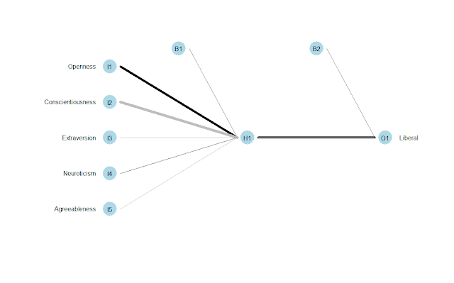
This post is a demonstration using the caret and nnet packages on aggregate Big Five traits per state and political leanings, and a continuation of a series: Neural Networks (Part 1 of 4) - Logistic Regression and neuralnet on State 'Personality' and Political Outcomes Neural Networks (Part 2 of 4) - caret and nnet on State 'Personality' and Political Outcomes This process using a neural net process to train then test on data. The neural net itself would be envisioned as follows: Initially, the results seemed promising, with a prediction accuracy of ~.85, further analysis revealed that the bulk of accurate predictions were those that had no price change, and that price change classes were often inaccurate. I excluded security types without price change, and the average dropped even further. I then created a loop that calculated test and training data by security type, and those result indicated that the neural net very right and very wrong, for price change s...

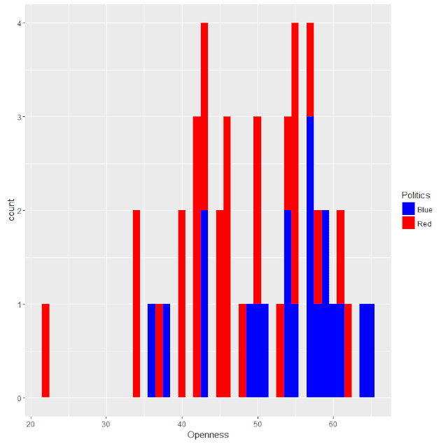
This is a continuation of a prior post, Neural Networks (Part 1 of 4) - Logistic Regression and neuralnet on State 'Personality' and Political Outcomes , the second in a series exploring neural networks. This post is a demonstration using the caret and nnet packages on aggregate Big Five traits per state and political leanings. Given the small sample size, there was a lower predictive ability using the train/test scenario using 80%, around .66, versus the entire set, which was correct at .83. This is evident in the graphs using lm() and stat_smoot(). The code is below, as are some related graphs. Source data is here . ################################################ # Neural Net with nnet and caret ################################################ # load packages library(nnet) library(caret) # train Politics.model <- train(equation, Politics.df, method = 'nnet', linout = TRUE, trace = FALSE) Politics.model.predicted <- predi...

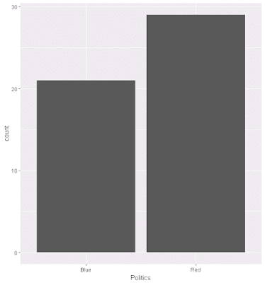
This is an example of neural networks using the neuralnet package on one of my sample data sets, walking through a Pluralsight training series, Data Mining Algorithms in SSAS, Excel, and R . In terms of results, the regression primarily predicts voter leanings based on five (5) traits, openness, conscientiousness, extraversion, agreeableness, and neuroticism, although only the first two (2) traits have a significant impact. Logistic regression is about 85% predictive, and slightly better at predicting Red states over its ability in predicting Blue states. [1] "Logistic Regression (All) - Correct (%) = 0.854166666666667" [1] "Logistic Regression (Red) - Correct (%) = 0.892857142857143" [1] "Logistic Regression (Blue) - Correct (%) = 0.8" For the neuralnet package, I created a loop to vary the hidden layers and the number of repetitions, since this is such a small number of records. This is obviously much less predictive than logistic regressi...

This is an example of Support Vector Machines, using one of my usual data sets, as part of a Pluralsight training presentation, Data Mining Algorithms in SSAS, Excel, and R . In terms of results, the prediction primarily predicts voter leanings based on two (2) traits, openness and conscientiousness, and although using all five (5) factors improved the prediction quality, plotting that is problematic. For this, the model is 96% predictive of Republican outcomes, but only 66% accurate in predicting Democratic leaning. Politics.prediction Blue Red Blue 15 1 Red 5 27 The code is below, as are some related graphs. Source data is here . # Clear memory rm(list = ls()) # set Working directory getwd() setwd('../Data') # load data Politics.df <- read.csv("BigFiveScoresByState.csv", na.strings = c("", "NA")) # clean data - remove NULLs Politics.df <- na.omit(Politic...

I noticed this very simple, very powerful article by James Marquez, Seven Easy Graphs to Visualize Correlation Matrices in R , in the Google+ community, R Programming for Data Analysis , so thought to give it a try, since I started some of my current analyses a decade ago by generating correlation matrices in Excel, which I've sometimes redone and improved in R. Some of these packages are only designed for display, or as extensions to ggplot2: corrplot: Visualization of a Correlation Matrix GGally: Extension to 'ggplot2' ggcorrplot: Visualization of a Correlation Matrix using 'ggplot2' These two are focused on more complex analysis: PerformanceAnalytics: Econometric tools for performance and risk analysis psych: Procedures for Psychological, Psychometric, and Personality Research As for data, I used Hofstede's culture dimensions, limited to developed countries. Using a broader and larger set of of countries would significantly reduce the correlation...

This decision tree demo is similar to a prior one I've done, but in this case, it uses the party package, that produces much higher-quality graphics than rpart, at least when used with plot. Although the idea for this analysis is mine, this was done as part of work for a Pluralsight training presentation, Data Mining Algorithms in SSAS, Excel, and R . Source data is here . # # Load Data # # Set working directory setwd("../Data") getwd() # read from data frame BigFivByState.df <- read.table("BigFiveScoresByState.csv", header = TRUE, sep = ",") # # Run Analysis # # Load package, install.packages('party', dependencies = TRUE) library(party) # train the model BigFivByState.dt <- ctree(data = BigFivByState.df, Liberal ~ Openness + Conscientiousness + Extraversion + Neuroticism + Agreeableness) # plot result plot(BigFivByState.dt, uniform = TRUE, main = ...

As part of another Pluralsight training presentation, Data Mining Algorithms in SSAS, Excel, and R , I worked through various exercises, and from that I've adapated Naive Basyes to one of my existing data sets. The code is below, as are some related graphs. Overall, the percent correct predicted based on Big Five personality traits using the Naive Bayes calculation is 66%. Source data is here . # # Load & Explore Data # # read from data frame BigFivByState.df <- read.table("BigFiveScoresByState.csv", header = TRUE, sep = ",") # review data head(BigFivByState.df) nrow(BigFivByState.df) summary(BigFivByState.df) names(BigFivByState.df) # various aggregations # as "count this value" ~ grouped by this + this Liberal.dist <- aggregate(State ~ Liberal, data = BigFivByState.df, FUN = length) head(Liberal.dist) RedBlue.dist <- aggregate(State ~ Politics, data = BigFivByState.df, FU...

As part of a Pluralsight training presentation, Understanding and Applying Logistic Regression , students worked through various exercises, one of which was predicting stock price changes, up or down, on Google, using Google and Spyder closing prices. As an ordered list of actions: Load data - Yahoo financials for each day for 5 years, taking only date and closing price for this analysis Transform sources: Merge sources, change column headings, cast the Date column as DATE type, sort descending Perform logistic regression Create a frame of actual versus predicted changes, and add a column for the correct/incorrect prediction result Find percent correct, on whether the price moved correctly up or down As a result, the lagged Google and SPY prices accurately predict next day prices about 63% of the time. Source data is here . # Clear memory rm(list = ls()) # Set working directory setwd("../Data") getwd() # load data # Data is Yahoo finan...