Multiple Regression with R, on IQ for Gini and Linguistic Diversity
Similar to the post about linear regression, Linear Regression with R, on IQ for Gini and Linguistc Diversity, this the same data used for multiple regression, with some minor but statistically significant examples:
Example Code
Example Results
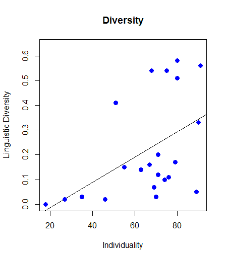
Example Plot
Sample Data
Example Code
 # LM - Multiple Regression

 # Load the data into a matrix
 oecdData <- read.table("OECD - Quality of Life.csv", header = TRUE, sep = ",")
 print(names(oecdData))
 # Access the vectors
 v1 <- oecdData$IQ
 v2 <- oecdData$HofstederPowerDx
 v3 <- oecdData$HofstederMasculinity
 v4 <- oecdData$HofstederIndividuality
 v5 <- oecdData$HofstederUncertaintyAvoidance
 v6 <- oecdData$Diversity_Ethnic
 v7 <- oecdData$Diversity_Linguistic
 v8 <- oecdData$Diversity_Religious
 v9 <- oecdData$Gini

 # Gini ~ Hofstede
 relation1 <- lm(v9 ~ v2 + v3 + v4 + v5)
 print(relation1)
 print(summary(relation1))
 print(anova(relation1))

 # IQ ~ Hofstede Individuality, Linguistic Diversity
 relation1 <- lm(v1 ~ v4 + v7)
 print(relation1)
 print(summary(relation1))
 print(anova(relation1))
Example Results
 > # Load the data into a matrix
 + oecdData <- read.table("OECD - Quality of Life.csv", header = TRUE, sep = ",")
 +
 + # Access the vectors
 + v1 <- oecdData$IQ
 + v2 <- oecdData$HofstederPowerDx
 + v3 <- oecdData$HofstederMasculinity
 + v4 <- oecdData$HofstederIndividuality
 + v5 <- oecdData$HofstederUncertaintyAvoidance
 + v6 <- oecdData$Diversity_Ethnic
 + v7 <- oecdData$Diversity_Linguistic
 + v8 <- oecdData$Diversity_Religious
 + v9 <- oecdData$Gini
 +
 + # Gini ~ Hofstede
 + relation1 <- lm(v9 ~ v2 + v3 + v4 + v5)
 + print(relation1)
 + print(summary(relation1))
 + print(anova(relation1))
 +
 + # IQ ~ Hofstede Individuality, Linguistic Diversity
 + relation1 <- lm(v1 ~ v4 + v7)
 + print(relation1)
 + print(summary(relation1))
 + print(anova(relation1))

 Call:
 lm(formula = v9 ~ v2 + v3 + v4 + v5)

 Coefficients:
 (Intercept)      v2      v3      v4      v5
   25.87750   0.10809   0.07172   0.01641   -0.04880


 Call:
 lm(formula = v9 ~ v2 + v3 + v4 + v5)

 Residuals:
   Min   1Q Median   3Q   Max
 -9.8929 -2.6618 0.2999 2.5365 8.2216

 Coefficients:
       Estimate Std. Error t value Pr(>|t|)
 (Intercept) 25.87750  8.36212  3.095 0.00658 **
 v2      0.10809  0.12080  0.895 0.38342
 v3      0.07172  0.05201  1.379 0.18582
 v4      0.01641  0.08473  0.194 0.84871
 v5     -0.04880  0.10407 -0.469 0.64509
 ---
 Signif. codes: 0 ‘***’ 0.001 ‘**’ 0.01 ‘*’ 0.05 ‘.’ 0.1 ‘ ’ 1

 Residual standard error: 4.967 on 17 degrees of freedom
  (3 observations deleted due to missingness)
 Multiple R-squared: 0.1497,     Adjusted R-squared: -0.05035
 F-statistic: 0.7483 on 4 and 17 DF, p-value: 0.5726

 Analysis of Variance Table

 Response: v9
      Df Sum Sq Mean Sq F value Pr(>F)
 v2     1 10.28 10.277 0.4166 0.5273
 v3     1 45.83 45.827 1.8577 0.1907
 v4     1 12.31 12.312 0.4991 0.4895
 v5     1  5.42  5.424 0.2199 0.6451
 Residuals 17 419.36 24.668

 Call:
 lm(formula = v1 ~ v4 + v7)

 Coefficients:
 (Intercept)      v4      v7
  100.21289   -0.02029   1.78454


 Call:
 lm(formula = v1 ~ v4 + v7)

 Residuals:
   Min   1Q Median   3Q   Max
 -7.5562 -1.2709 -0.2722 2.3429 6.1523

 Coefficients:
        Estimate Std. Error t value Pr(>|t|)
 (Intercept) 100.21289  2.74669 36.485  <2e-16 ***
 v4      -0.02029  0.04525 -0.448  0.659
 v7      1.78454  4.33483  0.412  0.685
 ---
 Signif. codes: 0 ‘***’ 0.001 ‘**’ 0.01 ‘*’ 0.05 ‘.’ 0.1 ‘ ’ 1

 Residual standard error: 3.563 on 19 degrees of freedom
  (3 observations deleted due to missingness)
 Multiple R-squared: 0.01297,     Adjusted R-squared: -0.09093
 F-statistic: 0.1248 on 2 and 19 DF, p-value: 0.8834

 Analysis of Variance Table

 Response: v1
      Df  Sum Sq Mean Sq F value Pr(>F)
 v4     1  1.018  1.0175  0.0802  0.7802
 v7     1  2.151  2.1514  0.1695  0.6852
 Residuals 19 241.195 12.6945
 >
Example Plot

Sample Data


Comments
Post a Comment