Hofstede's Long-term Orientation and Individuality: Obesity Relationships (using R)

Hofstede extended his original four dimensions, adding measures Long-Term Orientation (LTO) and Indulgence (Ind) in response to other researchers studies. While reading Hofstede's Cultures and Organizations: Software of the Mind, Third Edition I was struck by the lackluster reporting of the correlation between obesity and indulgence. It seemed obvious one would delve a bit further, maybe looking at a compound relationship between both indulgence and LTO, e.g., does short-sightedness and indulgence lead to obesity. Although I limit my analysis to OECD countries, that is what I present here.

An explanation of dimensions can be found on Hofstede's site.

Hofstede's Dimensions and Obesity

A first step would be to see what relationships exist between obesity and the dimensions:

1:  # LM - Multiple Regression - New Hofstede, LTO and Ind  
2:  # Load the data into a matrix  
3:  rm(list = ls())  
4:  setwd("../Data")  
5:  oecdData <- read.table("OECD - Quality of Life.csv", header = TRUE, sep = ",")  
6:  print(names(oecdData))  
7:    
8:  # Access the vectors  
9:  v1 <- oecdData$IQ  
10:  v2 <- oecdData$HofstederPowerDx  
11:  v3 <- oecdData$HofstederMasculinity  
12:  v4 <- oecdData$HofstederIndividuality  
13:  v5 <- oecdData$HofstederUncertaintyAvoidance  
14:  v6 <- oecdData$HofstederLongtermOrientation  
15:  v7 <- oecdData$HofstederIndulgence  
16:    
17:  v9 <- oecdData$Gini  
18:  v10 <- oecdData$Obesity  
19:  v26 <- oecdData$Assaultsandthreats  
20:    
21:  # Conclusion, both high individuality and low LTO contribute to obesity  
22:  #  but inversely correlated with each other  
23:  # Obesity ~ Hofstede  
24:  relation1 <- lm(v10 ~ v2 + v3 + v4 + v5 + v6 + v7)  
25:  print(relation1)  
26:  print(summary(relation1))  
27:  print(anova(relation1))  

Results - Regression and ANOVA

Both linear multiple regression and ANOVA would indicate that both individuality and LTO have, or at least one has, a relationship to obesity.

1:  Call:  
2:  lm(formula = v10 ~ v2 + v3 + v4 + v5 + v6 + v7)  
3:    
4:  Coefficients:  
5:  (Intercept)      v2      v3      v4      v5      v6      v7   
6:    1.09265   0.12813   0.07237   0.10560   -0.01969   -0.14108   0.08111   
7:    
8:  Call:  
9:  lm(formula = v10 ~ v2 + v3 + v4 + v5 + v6 + v7)  
10:    
11:  Residuals:  
12:    Min   1Q Median   3Q   Max   
13:  -5.3248 -3.1639 -0.1943 1.3526 9.3436   
14:    
15:  Coefficients:  
16:        Estimate Std. Error t value Pr(>|t|)   
17:  (Intercept) 1.09265  11.38472  0.096  0.9247   
18:  v2      0.12813  0.12105  1.059  0.3055   
19:  v3      0.07237  0.04969  1.456  0.1646   
20:  v4      0.10560  0.09187  1.150  0.2672   
21:  v5     -0.01969  0.10441 -0.189  0.8528   
22:  v6     -0.14108  0.05303 -2.660  0.0171 *  
23:  v7      0.08111  0.12755  0.636  0.5338   
24:    
25:  Signif. codes: 0 `***' 0.001 `**' 0.01 `*' 0.05 `.' 0.1 ` ' 1  
26:    
27:  Residual standard error: 4.715 on 16 degrees of freedom  
28:   (1 observation deleted due to missingness)  
29:  Multiple R-squared: 0.5731,     Adjusted R-squared: 0.4131   
30:  F-statistic: 3.581 on 6 and 16 DF, p-value: 0.01919  
31:    
32:  Analysis of Variance Table  
33:    
34:  Response: v10  
35:       Df Sum Sq Mean Sq F value  Pr(>F)    
36:  v2     1 26.81 26.814 1.2059 0.288389    
37:  v3     1 17.73 17.731 0.7974 0.385093    
38:  v4     1 253.50 253.495 11.4008 0.003846 **  
39:  v5     1  5.22  5.217 0.2346 0.634672    
40:  v6     1 165.43 165.431 7.4402 0.014902 *   
41:  v7     1  8.99  8.990 0.4043 0.533847    
42:  Residuals 16 355.76 22.235            
43:    
44:  Signif. codes: 0 `***' 0.001 `**' 0.01 `*' 0.05 `.' 0.1 ` ' 1  

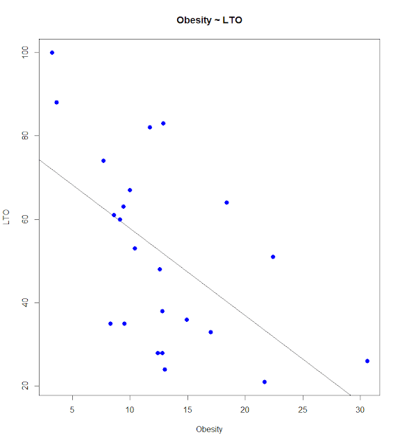
Correlations and Graphs - LTO and Obesity

1:  # Corr - Obesity ~ LTO  
2:  cor.test(v6, v10)  
3:  plot(v10, v6, col = "blue", main = "Obesity ~ LTO", abline(lm(v6 ~ v10)), cex = 1.3, pch = 16, xlab = "Obesity", ylab = "LTO")  
    

The results seem significant, with a correlation of -.56.

1:  Pearson's product-moment correlation  
2:    
3:  data: v6 and v10  
4:  t = -3.1025, df = 21, p-value = 0.005392  
5:  alternative hypothesis: true correlation is not equal to 0  
6:  95 percent confidence interval:  
7:   -0.7902136 -0.1930253  
8:  sample estimates:  
9:      cor   
10:  -0.5606214   
    

Correlations and Graphs - Individuality and Obesity

1:  # Corr - Obesity ~ Idv  
2:  cor.test(v4, v10)  
3:  plot(v10, v4, col = "blue", main = "Obesity ~ Idv", abline(lm(v4 ~ v10)), cex = 1.3, pch = 16, xlab = "Obesity", ylab = "Idv")  

These results seem equally significant, with a correlation of .59.

1: Pearson's product-moment correlation  
2:    
3:  data: v4 and v10  
4:  t = 3.351, df = 21, p-value = 0.003027  
5:  alternative hypothesis: true correlation is not equal to 0  
6:  95 percent confidence interval:  
7:   0.2353225 0.8062918  
8:  sample estimates:  
9:     cor   
10:  0.5902683   

Concern - Correlation between Individuality and LTO

Although the two qualities are not linearly related, they have a significant degree of correlation, -.33.


Sample Data